Wolves may have domesticated themselves by scavenging human scraps. A mathematical method called adaptive dynamics tests whether this proto-domestication idea holds up.
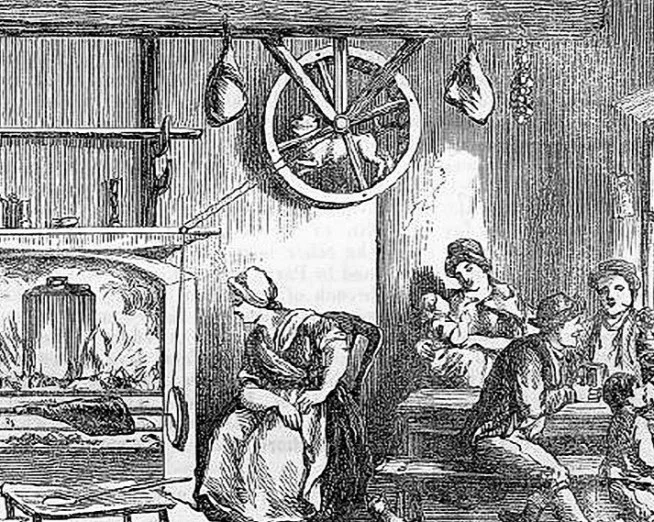
Dogs are the oldest domesticated animal we know of, and they've been shaped by people for thousands of years. The result is a range of body types and temperaments that few other species can match. Some breeds herd and guard livestock. Others hunt, tracking, chasing, or retrieving game. Working dogs rely on their noses or their sturdy builds, and service dogs help people with disabilities live more independently. Not long ago, one breed even existed purely to turn a wheel, often to drive kitchen equipment. The turnspit was bred for that single job. So how did a wild predator end up doing all of this?
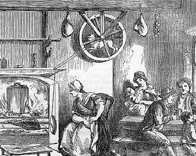
Turnspit dogs ran in wheels to turn meat, depicted here in a Welsh pub in 1797.
Breeders have been selecting for these jobs for centuries, and that part is well documented. The harder question is how we first got animals this tame. We know dogs evolved from prehistoric grey wolves, and grey wolves are still with us. At some point, one lineage split off. Some wolves stayed wild, while others eventually became the animals that live in our homes. Nobody knows for certain what pushed that split, and researchers have proposed several explanations.
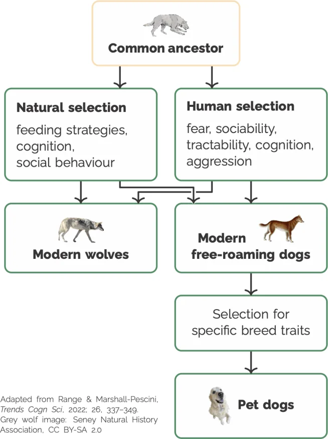
The domestication process. (Source)
One idea is that wolves and early humans hunted in complementary ways, and that cooperation grew out of it. Another is that people raised wolf pups by hand. A pup raised this way bonds with its carer early, and that bond becomes the foundation. Over generations, the aggressive animals were weeded out, and the sociable ones were kept and bred, each round producing tamer descendants. The third explanation has the most traction, and it's the most interesting to me. It's called proto-domestication, and the idea is that wolves domesticated themselves. The less fearful ones could live off human scraps, which were a more dependable meal than hunting wild prey.
Here's where it gets fun. You can test these ideas with mathematics. This piece uses a method called adaptive dynamics to check whether proto-domestication holds up as a model.
What adaptive dynamics actually does
Adaptive dynamics applies natural selection to the parameters that drive a population's dynamics. The core assumption is that traits giving an individual an advantage will spread. A mutant trait succeeds if it grows faster than the trait already present in the population.
Before going further, the method rests on a few simplifications that you need to accept. They're standard in the field, and you can read about them in these references on the method.
- Mutations are small: a mutant individual doesn’t differ much from its parent.
- Mutations are rare: The number of mutants that arise at any one time is very small. This allows us to approximate the total population with the resident population (the one in place before any mutations).
- The evolutionary timescale is much larger than the dynamical system timescale. The population is allowed to reach equilibrium between successive mutations.
The method also tracks one evolutionary trait at a time. For wolves, that trait is friendliness, tameness, or something close to it. The justification comes from Dmitri Belyaev's fox experiments, which started in the 1950s. He found that tameness came bundled with other changes: floppier ears, softer features, shorter snouts, and smaller bodies. Those features tended to show up on their own among the friendlier animals. That's convenient. You don't have to model each physical change separately, because one dial, friendliness, carries most of the signal. Belyaev's work is covered in this account of the fox experiment.
Starting at $f=0$
The friendliness trait becomes a parameter $f\in[0,1]$ in the model of the prehistoric wolf population. At $f=0$, the wolves are fully wild and avoid humans. They're good hunters, and they gain nothing from scraps. At $f=1$, the wolves are as tame as the standard set before selective breeding began. They tolerate people, so they can eat from human settlements.
Because the population is made of wolves, a classic Lotka–Volterra model is a sensible starting point. That model is usually applied to predators and prey. Here, though, the interest is in how different wolf types interact with one another, not with their prey.
Consider two sub-populations of wolves with different friendliness. The first, $W$, grows in proportion to its current size. Its growth is held back by competition with itself and with the second sub-population, $W’$:
\begin{equation*} \frac{\mathrm{d}{W}}{\mathrm{d}t} = \underbrace{rW}_{{\text{growth}}} – \underbrace{\frac{r}{K}W^2}_{{\substack{\text{self-}\\\text{competition}}}} – \underbrace{cWW’}_{{\text{with }W’}}. \end{equation*}
In this equation, $r$ is the familiar growth rate, which captures breeding success and litter size. $K$ is the carrying capacity of $W$, meaning the population it would settle at without any other sub-populations present.
Extending this to many sub-populations, each with its own $f$, gives (after some relabelling)
\begin{equation*} \frac{\mathrm{d}W(f,t)}{\mathrm{d}t} = rW(f,t)\left[1\!-\!\sum_{f’}\frac{\alpha(f-f’)W(f’,t)}{K(f)}\right]. \label{pop_density} \end{equation*}
The function $\alpha(f-f’)$ measures how much a wolf with friendliness $f’$ competes with one at $f$. It takes a Gaussian form:
\begin{equation*} \alpha(f-f’) = \exp{\left(\frac{-(f-f’)^2}{2\sigma_\alpha^2}\right)}. \label{branch_comp} \end{equation*}
The logic is intuitive. Wolves with similar temperaments fight over the same resources, so they compete hard. Wolves that differ a lot barely interfere. Wild wolves chase the same prey, and tame ones crowd around the same scraps. The width $\sigma_\alpha$ sets how far that rivalry reaches. The two curves below show how the width changes the picture.
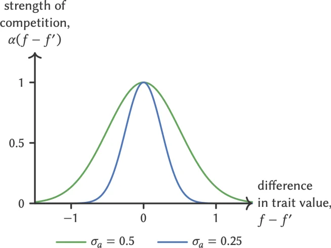
We can use Gaussian distributions to represent the competition exerted by the trait $f’$ on the trait $f$ by the difference $f-f’$. The two widths, $\sigma_\alpha$, represent different spreads of trait values.
The carrying capacity $K(f)$ needs more care, because it has to reflect two very different food sources. Wild prey sits at one end, and human scraps sit at the other. The model uses a double Gaussian, with one peak at $f=0$ (wild) and one at $f=1$ (docile):
\begin{equation*} K(f) = \underbrace{A\exp{\left(\frac{-f^2}{2\sigma_\text{w}^2}\right)}}_{{\text{wild resource}}} + \underbrace{B\exp{\left(\frac{-(f-1)^2}{2\sigma_\text{d}^2}\right)}}_{{\text{human resource}}}. \end{equation*}
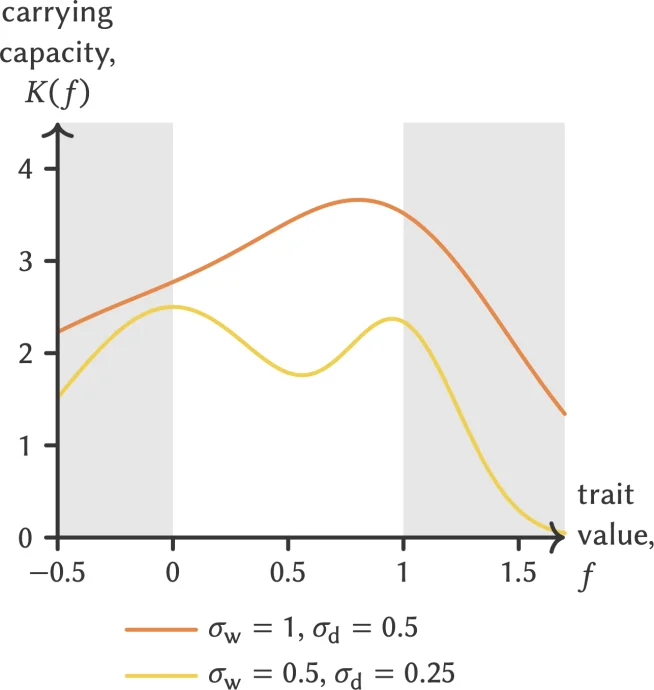
The carrying capacity of the wolf population varies with trait value $f$ and the niche widths $\sigma_\text{w}$ and $\sigma_\text{d}$. Each hump indicates trait values that promote the highest equilibrium population densities. Shading excludes impossible values of $f$. Here, $A=2.5$ and $B=2$.
Narrow widths make the two food sources distinct, and you get two separate peaks. That's the model's version of a lesson about specialisation: it pays to be an expert rather than a jack of all trades. The wildest wolves hunt best, and as friendliness rises, hunting skill drops. The boldest tame wolves get first pick of human scraps, which leaves less for the cautious ones.
The reverse holds too. Wolves that do poorly against wild prey are the ones more likely to drift toward self-domestication. That's a useful intuition, and it's the core of the whole argument.
Widen the spreads, though, and the two food sources overlap heavily. The peaks merge, and a single best compromise emerges somewhere between wild and human resources.
Which wolf wins?
With the model set up, the adaptive dynamics analysis can begin. The resident trait is $f=x$, the value before any mutation. The placeholder for a mutant is $f=y$.
Under the method's assumptions, a rare mutant means the mutant population $W’ = W(y,t)$ is effectively zero at first. A long evolutionary timescale lets the resident population settle at its equilibrium value, $W^*(x)$. Setting $\frac{\mathrm{d}W(x,t)}{\mathrm{d}t}=0$ and using the resident-only version of the equation gives
\begin{align*} rW^*(x)\left[1-\frac{\alpha(x-x)W^*(x)}{K(x)}\right] &= 0 \\ \implies W^*(x) &= K(x). \label{eqn:residentdensity} \end{align*}
The first real test asks whether a mutant, one slightly more or less human-tolerant than its pack, can succeed when everyone else shares the same friendliness. The measure for this is the invasion fitness. The hitchhiker’s guide to adaptive dynamics defines it as the expected per capita growth rate of a rare mutant in the environment the resident population creates.
Written as $F_x(y)$, with $x$ the resident and $y$ the mutant, it works out to
\begin{align*} F_x(y) &= \left.\frac{1}{W(y,t)}\frac{\mathrm{d}W(y,t)}{\mathrm{d}t}\right|_{\begin{subarray}{l}W(x,t)=W^*(x)=K(x),\\W(y,t)=0\end{subarray}}\\ &= r\left[1-\frac{\alpha(y-x)K(x)+\alpha(x-x)\cdot 0}{K(y)}\right]\\ &= r\left[1-\frac{\alpha(y-x)K(x)}{K(y)}\right]. \end{align*}
The sign is what matters. A positive invasion fitness means the mutant takes hold. A negative one means it dies out.
The plot below takes three resident traits, $x=0.2$ (pink), $0.5$ (purple) and $0.8$ (blue), representing mostly wild, intermediate and mostly docile wolves.
There's a neat consequence here. $F_x(x)=0$ always, so a mutant identical to the resident has no edge either way. The useful question is which direction from $x$ leads somewhere better. The answer is whichever side gives a positive value.
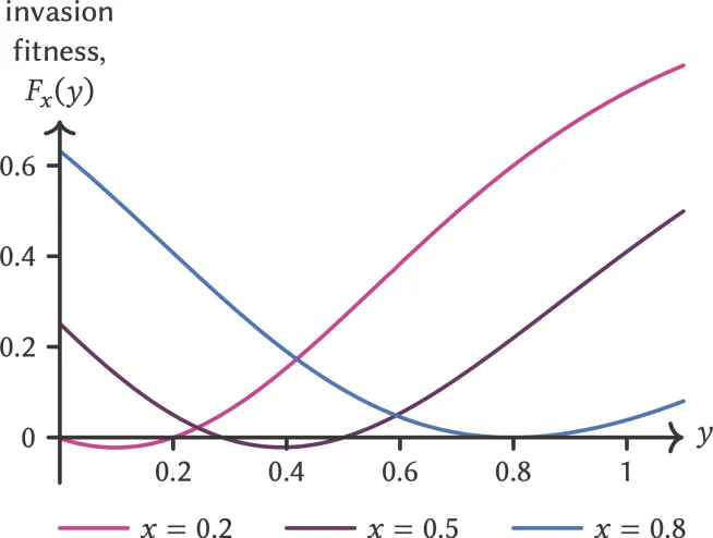
Given the carrying capacity, $K(f)$, shown above with $\sigma_\text{w}=1,\sigma_\text{d}=0.5$ (orange), here are three plots of the invasion fitness, $F_x(y)$, for different resident traits, $x$. Notice that $F_x(x)=0$ in every case: if the mutant is the same as the resident trait, there will be no (dis)advantage. The strength of competition width is $\sigma_\alpha=0.5$.
Sign tells you a lot, but it's easier to see on a pairwise invasibility plot (PIP). It maps the sign of $F_x(y)$ across every pairing of resident and mutant trait. The PIP below shows exactly that.
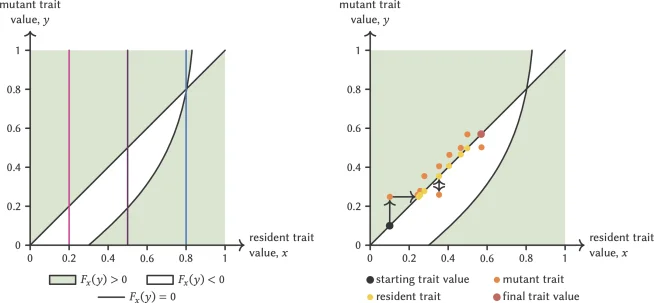
Plots of mutant trait value by resident trait value. Green regions show where the invasion fitness is positive; white regions are negative. The regions are separated by black contours of $F_x(y)=0$. The left-hand plot shows that the curves of fixed $x$ from the previous graph exhibit the same invasion fitness polarity. The right-hand plot shows how traits will evolve along the diagonal: if a mutant trait is in the green region it will be successful and the population will evolve to adopt this new trait. But if it lies in the white region, the resident trait will remain the same. This evolution sequence is shown for a limited number of mutations but the pattern shows evolution will continue towards the point where the contours intersect. Parameters: $A=2.5$, $B=2$, $\sigma_\text{w} = 1$, $\sigma_\text{d} = 0.5$ and $\sigma_\alpha = 0.6$.
The mutations-are-small assumption opens a second route. Instead of checking distant mutants, you can look at the slope of the fitness curve at $y=x$. That slope is the selection gradient:
\begin{align*} s(x) &= \left.\frac{\partial F_x(y)}{\partial y}\right|_{y=x} \\ &=r\,\Biggl[-\underbrace{\left.\frac{\partial \alpha(y-x)}{\partial y}\right|_{y=x}}_{=\;0} + \frac{\partial K(x)}{\partial x}\frac{1}{K(x)}\Biggr]\\ &=\frac{r}{K(x)}\frac{\partial K(x)}{\partial x}. \end{align*}
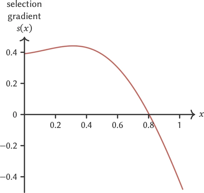
The selection gradient, $s(x)$, for the resident trait, $x$, tells us whether friendlier or less friendly mutants are favoured for each $x$. This plot is based
on the carrying capacity from above with $\sigma_\text{w} = 1$, $\sigma_\text{d} = 0.5$.
The gradient carries two pieces of information: how fast evolution moves and which way it goes. A positive $s$ favours slightly friendlier mutants. A negative $s$ favours slightly less friendly ones. Put another way, if the PIP is green above the diagonal and white below, a friendlier wolf does better, so $s(x)>0$ and the population climbs up and to the right. The reverse gives $s(x)<0$, and the population slides down and to the left.
The singular strategy, and where wolves split
The interesting case sits where $s(x^*)=0$. Here, neither friendlier nor wilder mutants win out. This point is the evolutionarily singular strategy, and on the PIP it appears where the $F_x(y)=0$ contours cross.
Interesting, though, can mean several things. What I care about is a singular strategy that's also a branch point. A branch point does two things at once. It pulls evolution toward itself, which is convergence, and it then pushes the population apart into distinct groups heading to different trait values, which is instability.
Convergence requires $s'(x^*) < 0$. Instability requires that $F_{x^*}(y)$ has a local minimum at $y=x^*$, so any mutation away from $x^*$ grows. Working through the algebra shows that both conditions amount to the inequality
\begin{alignat*}{3} \left.\frac{\partial^2 F_x(y)}{\partial x^2}\right|_{y=x=x^*} &>\;& \left.\frac{\partial^2 F_x(y)}{\partial y^2}\right|_{y=x=x^*} &>0. \end{alignat*}
For this model, that becomes
\begin{equation*}\begin{split} r\left(\frac{1}{\sigma_\alpha^2} – \frac{1}{K(x^*)}\left.\frac{\partial^2 K(x)}{\partial x^2}\right|_{x=x^*}\right) \hspace{2cm} \\ > r\left(\frac{1}{\sigma_\alpha^2} + \frac{1}{K(x^*)}\left.\frac{\partial^2 K(x)}{\partial x^2}\right|_{x=x^*}\right) >0. \end{split} \end{equation*}
Now test it on the wolves. Candidate singular strategies come from solving $\frac{\partial K(x)}{\partial x}=0$, which means finding the stationary points of the carrying capacity. That step has to be done numerically.
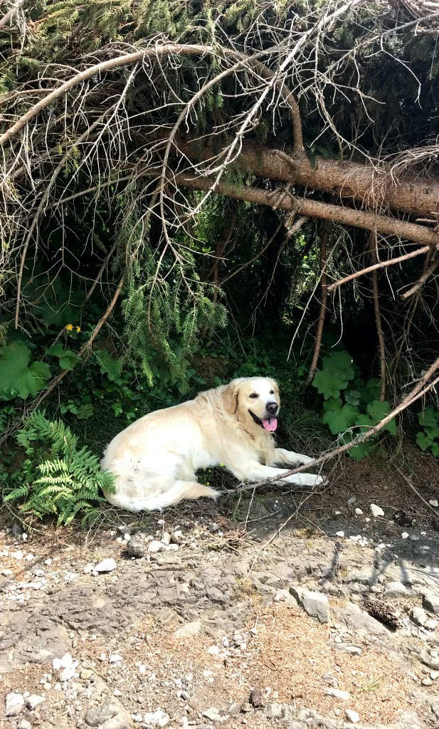
Benji’s favourite branch point is under one, in the shade. (Benji, $f=1$, will happily eat human scraps.)
The stability condition is where the model's conclusion gets decided, so it's worth slowing down on. For the population to converge, the second derivative of $K(x)$ at $x^*$ has to be negative: \begin{equation*} \left.\frac{\partial^2 K(x)}{\partial x^2}\right|_{x=x^*} < 0, \end{equation*} which means every branch point has to be a maximum of $K(f)$. Once that's in place, the instability condition only holds when \begin{align*} \frac{K(x^*)}{\sigma_\alpha^2} > &-\left. \frac{\partial^2 K(x)}{\partial x^2}\right|_{x=x^*} = \left| \frac{\partial^2 K(x)}{\partial x^2}\right|_{x=x^*}\\ \implies&\frac{K(x^*)}{\hspace{2em}\left|\frac{\partial^2 K(x)}{\partial x^2}\right|_{x=x^*}} > \sigma_\alpha^2. \end{align*} Both sides are positive, so the inequality can be satisfied, but only when the wolf–wolf competition width is narrow enough. That's the key constraint. Narrow competition is what lets a branch form at all.
Look back at the $K(f)$ plots and you'll see there are two ways this can happen.
Case 1, the yellow curve, has narrow niche widths and a branch point near $f=0$. This is the one that matters for the domestication story. Every wolf starts out wild, living off wild resources, so a split close to zero is where the process begins.
Case 2, the orange curve, has wide niche widths and a branch point at a mid-range friendliness value. Both cases show up in stochastic simulations, provided the parameters satisfy the branching constraints derived earlier. The simulations are on the next page.
Which case is more realistic? The plots point to Case 1, though Case 2 is deliberately extreme. Changing $A$, $B$, $\sigma_\text{w}$ and $\sigma_\text{d}$ moves the branch point toward zero, which is where the real branch is more likely to sit. That's useful, because it means the model isn't simply tuned to produce the answer it wants.
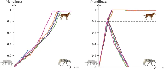
Stochastic simulations of friendliness evolution in prehistoric wolves over time. Values of $\sigma_\alpha$ are chosen so that both cases satisfy the conditions for a branch point near $0$. Each coloured curve is a separate realisation, showing the pattern isn't a one-off. In both cases one branch drifts into purely wild wolves, while the other grows friendlier until it becomes domestic enough for selective breeding to take over. That final step would need a separate model. Parameters: $A=2.5$, $B=2$, maximum mutational step $=0.01$. Case 1: $\sigma_\text{w} = 0.5$, $\sigma_\text{d}=0.25$, $\sigma_\alpha = 0.4$. With humans present, the population branches at a value of $f$ very close to zero. Case 2: $\sigma_\text{w} = 1$, $\sigma_\text{d}=0.5$, $\sigma_\alpha = 0.6$. With humans present, the population becomes friendlier until a critical value is reached, then splits into increasingly wild and increasingly friendly wolves. Images: Grey wolf image, Seney Natural History Association, CC BY-SA 2.0.
Why the split happens at zero
Here's the thing: the parameter regime that looks most plausible also has the most satisfying biological reading. We'd expect $A$ to be much larger than $B$ early on, meaning the purely wild wolf population could support far more individuals than a purely domestic one. Under those conditions the branch point lands very near zero, whatever case you're in.
That matters because grey wolves are essentially the direct descendants of prehistoric wolves. The model's preferred outcome has the population splitting right at $f=0$. Dogs diverge at that point and the wolves are left largely unchanged. The alternative would be a whole population drifting toward docility and then reversing course after the split. The model doesn't favour that path.
What the wolves tell us
So what did the maths actually show? For the model set up at the start, the benefit of human scraps is enough to drive prehistoric wolves toward becoming dogs and grey wolves. That supports the proto-domestication theory, at least within the model's assumptions.
The more interesting finding is what didn't happen. The wild population didn't disappear. Evolution wasn't a one-way street toward friendliness. Instead the model produces two distinct populations sharing the same geography. That cuts against a common assumption. Speciation is usually linked to geographic separation, with each population adapting to a different environment. These wolves didn't need that separation to split, and that's a finding worth pausing on.
There's also a broader point here. Mathematics earns its keep where data and experiments can't reach. Nobody can rerun the domestication of wolves, because it happened tens of thousands of years ago. A well-built model is one of the few tools left for asking what could have happened and under which conditions.
That said, the model doesn't settle the question. We still don't have a concrete answer for where our four-legged friends came from. What this work offers is one more piece of the puzzle, and a reasonably convincing one.



Discussion
Sign in to join the discussion.