— 1. The Hilbert transform — In this set of notes we begin the theory of singular integral operators – operators which are almost integral operators, except that their kernel just barely fails to be i...

— 1. The Hilbert transform —
In this set of notes we begin the theory of singular integral operators – operators which are almost integral operators, except that their kernel  just barely fails to be integrable near the diagonal
 . (This is in contrast to, say, fractional integral operators such as
 , whose kernels go to infinity at the diagonal but remain locally integrable.) These operators arise naturally in complex analysis, Fourier analysis, and also in PDE (in particular, they include the zeroth order pseudodifferential operators as a special case, about which more will be said later). It is here for the first time that we must make essential use of cancellation: cruder tools such as Schur’s test which do not take advantage of the sign of the kernel will not be effective here.
Before we turn to the general theory, let us study one of the simplest non-trivial singular integral operators, the Hilbert transform

 is well-defined even for nice functions
 . But if is
 and compactly supported, then we can restrict the integral to a compact interval
 for some large
 (depending on
 and ), and use symmetry to write

 is uniformly bounded on the interval for fixed
 , and so the limit actually exists from the dominated convergence theorem. A variant of this argument shows that
 is also well-defined for in the Schwartz class, though it does not map the Schwartz class to itself. Indeed it is not hard to see that we have the asymptotic
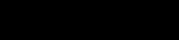
has non-zero mean then only decays like  at infinity. In particular, we already see that
 is not bounded on
 . However, we do see that at least maps the Schwartz class to
 .
Let us first make comment on some algebraic properties of the Hilbert transform. It commutes with translations

 -normalized dilations


Exercise 1 Letbe a continuous linear operator which maps Schwartz functions to bounded continuous functions, and which commutes with translations and dilations as in (2). Show that
is a linear multiple of the Hilbert transform and the identity. (Hint: first establish the existence of a distribution
such that
for all
, and such that
is homogeneous of degree
. Restrict the action of
or
and show that
on these functions.) (The claim is also true if we relax
to
, the space of distributions, but this is a little trickier to prove.)
It is also formally skew-adjoint:
Exercise 2 Ifare compactly supported, show that

The Hilbert transform is connected to complex analysis (and in particular to Cauchy integrals) by the Plemelj formulae.
Proposition 3 (Plemelj formulae) Letobey a qualitative decay bound
(say – these conditions are needed just to make


Proof: By translation invariance we can take  . By taking complex conjugates we may assume that the
 sign is
 . Our task is then to show that

 and making the change of variables
 , we reduce to showing




Now suppose that not only obeys the hypotheses of the Plemelj formulae, but also extends holomorphically to the upper half-plane  and obeys the decay bound
 in this region. Then Cauchy’s theorem gives


 in this case. In particular, comparing real and imaginary parts we conclude that
 and
 . Thus for reasonably decaying holomorphic functions on the upper half-plane, the real and imaginary parts of the boundary value are connected via the Hilbert transform. In particular this shows that such functions are uniquely determined by just the real part of the boundary value.
The above discussion also strongly suggests the identity  . This can be made more manifest by the following Fourier representation of the Hilbert transform.
Proposition 4 Iffor (almost every)
. (Recall that
and so its Fourier transform is defined via density by Plancherel’s theorem.)

Proof: Let us first give a non-rigorous proof of this identity. Morally speaking we have

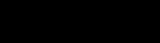

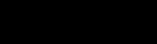
Now we turn to the rigorous proof. As the Hilbert transform is odd, a symmetry argument allows one to reduce to the case  . It then suffices to show that
 has vanishing Fourier transform in this half-line. Define the Cauchy integral operator

 as
 ; since is Schwartz, it is also not hard to show via dominated convergence that they also converge in . Thus by the boundedness of the Fourier transform it suffices to show that each of the
 also have vanishing Fourier transform on the half-line.
This is part of a more general phenomenon, that functions which extend holomorphically to the upper half-space in a controlled manner tend to have vanishing Fourier transform on , while those which extend to the lower half-space have vanishing Fourier transform on . Thus there is a close relationship between holomorphic extension and distribution of the Fourier transform.
Fix  (we could rescale
 to be, say,
 , but we will not have need of this normalization). We can truncate and define

 converges to
 in as
 and so it will suffice to show that the Fourier coefficients of converge pointwise to zero as on the half-line . From Fubini’s theorem we easily compute

and then letting  we obtain the claim.
From this proposition and Plancherel’s theorem we conclude that is an isometry:

has a unique dense extension to , and (by another application of Plancherel’s theorem to justify taking the limit) the formula (3) is valid for all  . There is still the question of whether the original definition is valid for , or in other words whether the sequence of functions
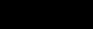
to for , and in what sense this convergence holds. It turns out that the convergence is true both pointwise almost everywhere and in the metric sense, and in fact it follows from variants of the Calderón–Zygmund theory presented in this notes, but we shall not do so here (as it may be covered in the participating student seminar).
From (3) we also see that we do indeed have the identity on , and that is indeed skew-adjoint on ( ); in particular, is unitary.
Let us briefly mention why the Hilbert transform is also connected to the theory of partial Fourier integrals, via the modulation operators

Proposition 5 Let. Then

Proof: By limiting arguments (and because everything is continuous on ) it suffices to verify this identity for in the Schwartz class. But then the claim follows by taking the Fourier transform of both sides and using (3).
It is thus clear that in order to address the question of the extent to which the partial Fourier integrals  actually converges back to , we will need to understand the properties of the Hilbert transform, and in particular its boundedness properties.
The formula (3) suggests that behaves “like” multiplication by  in some sense; informally, behaves like
 for positive frequency functions and
 for negative frequency functions. Now multiplication by is a fairly harmless operation – it is bounded on every normed vector space – so one might expect to similarly be bounded on more normed spaces than just ; in particular, it might be bounded on
 . This is indeed the case for
 , and we now turn to the theory which will generate such bounds.
Exercise 6 Demonstrate by example that the Hilbert transform is not bounded onor
.
— 2. Calderón–Zygmund theory —
In the Hilbert transform, we have an operator which is bounded on , and we wish to extend this boundedness to other spaces as well. This is of course not automatic – the “enemy” is that the operator might map a broad shallow function into a tall narrow function of comparable norm (which will increase the norms markedly for all  ), or conversely map a tall narrow function down to a broad shallow function of comparable norm (which will increase the norms markedly for
 ). It turns out that these two phenomena are more or less dual to each other, and so when working with an operator which is “comparable” to its adjoint (which is for instance the case with the skew-adjoint Hilbert transform, ) eliminating one of these enemies will automatically remove the other.
For operators such as the Hilbert transform, there are at least two approaches to exclude these scenarios. One is to exploit the phenomenon that if is not too large locally, then also doesn’t fluctuate too much locally; this prevents the “broad shallow to tall narrow” enemy which blocks boundedness for large  . The dual approach is to show that if is localized and fluctuating, then is also localized; this prevents the “tall narrow to broad shallow” enemy which blocks boundedness for small . (There are also more algebraic methods, relying on explicit formulae for things like the
 norm of , or of the size of level sets of
 for various sets
 , but we will not discuss those here as they do not extend well to the more general class of singular kernels considered here.)
We shall first discuss the latter approach, which is the traditional approach to the subject, and return to the former approach later. We shall generalize from the Hilbert transform to a useful wider class of operators, which are integral operators “away from the diagonal”. To motivate this concept, observe that if is compactly supported and  lies outside of the support of , then

is not, strictly speaking, an integral operator of the type studied in preceding sections, it can be described as such as long as one avoids the diagonal .
Definition 7 (Singular kernels) A singular kernel is a function(defined away from the diagonal
for
and the Hölder-type regularity estimates
and
for some Hölder exponent
.



Example 8 In one dimension,and
are both singular kernels. In higher dimensions, the kernel
is a singular kernel whenever
is a Hölder-continuous function.
The regularity estimates may seem strange at first sight, although the fundamental theorem of calculus shows that these estimates would follow (with  ) from the estimates

 is
 , these estimates are then consistent with (4) but of course do not follow from it. In most applications one can take
 (in which case the Hölder type conditions become Lipschitz type conditions). It is more desirable (5), (6) for large
 than for small (note in particular that the
 version of the estimate already follows from (4)). It is possible to weaken the Hölder type conditions further, but there are few applications that require such a weakening and so we shall stay with the Hölder condition. The factor
 is not significant; it is not hard to show that the regularity conditions are equivalent to the condition in which is replaced by any other constant strictly between zero and one.
Definition 9 (Calderón–Zygmund operators) A Calderón–Zygmund operator (CZO) is a linear operatorwhich is bounded on
,
and such that there exists a singular kernel
whenever
is compactly supported, and

It is not hard to see that uniquely determines . However the converse is not true; for instance, given any bounded function  , the physical space multiplier
 is a CZO with kernel
 . However, this is the only source of ambiguity; see Exercise 18. A CZO is an example of a singular integral operator; the kernel just barely fails to be locally integrable (Schur’s test, for instance, encounters a logarithmic divergence), and so there is a singularity in the integration which must be understood in order to analyze correctly. In particular, not all singular kernels lead to an CZO, due to possible failure of boundedness. We will return to the question of working out which kernels do give CZOs later.
Remark 10 As with the theory of the Hardy–Littlewood maximal function, one can define CZOs on more general homogeneous spaces than, but we will not do so here for sake of concreteness.
By convention, we allow all implied constants in what follows to depend on the Hölder exponent and on the implied constants in (4), (5), (6) and the operator norm bound on . (One could try to formalize things by imposing a norm on CZOs with a given exponent , but this gets a bit confusing and is largely unnecessary since one mostly deals with just a single CZO at a time.)
The Hilbert transform is thus a CZO, with kernel 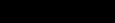 . We will discuss other examples of CZOs, such as the Riesz transforms, Hörmander–Mikhlin multipliers, and pseudodifferential operators of order zero, later on.
The Hilbert transform was skew-adjoint, translation-invariant, and scale-invariant. In general, CZOs are neither. However, the class of CZOs is self-adjoint (and skew-adjoint), translation-invariant, and scale-invariant; if is a CZO then so is  , and the translates
 and dilates
 of are also CZOs uniformly in
 and
 . (What happens to the kernels in each case?)
Now we formalize the key phenomenon alluded to earlier, that CZOs map fluctuating localized functions to nearly localized functions.
Lemma 11 Letbe a ball in
have mean zero, thus
. Then we have the pointwise bound
In particular, we have


Proof: We remark that we could use the translation and scaling symmetries of CZOs to normalize  , but we shall not do so here. For
 we can use the mean zero hypothesis to obtain

and  ).
Remark 12 Observe that the argument also gives the slightly more general estimatewhen the mean zero condition

This lemma asserts that is sort of bounded on – but only when the input function is localized and mean zero, and as long as one doesn’t look too closely at the region near the support of the function. This extremely conditional boundedness is a far cry from true boundedness; indeed, it is not hard to show that boundedness can fail. However, Lemma 11, combined with the Calderón–Zygmund decomposition from the previous section (which decomposes any function into a bounded part and a lot of localized, fluctuating parts) is strong enough to obtain the weak-type boundedness instead.
Corollary 13 All CZOs are of weak type, with an operator norm of
.
Proof: Let  (the condition ensuring that is well-defined), let be a CZO, and let . Our task is to show that
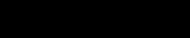
 and
 to both be ; this avoids a certain amount of book-keeping regarding these factors later. Applying the Calderón–Zygmund decomposition, we can split
 , where the “good” function
 obeys the bounds

 is supported on
 , has mean zero, and has the bound


 , we can split

boundedness of via Chebyshev’s inequality and log-convexity of Hölder norms: 
bounds because the have no reason to be bounded in . But the mean zero condition, combined with Lemma 11, shows that each  has bounds outside of a dilate
 of (for some fixed constant
 depending only on );

arbitrarily close to by iterating (5), (6) to obtain a variant of Lemma 11, but we will not do so here.).
Restricting to the common domain 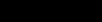 and summing in using the triangle inequality we obtain


 . But here is the great advantage of weak-type estimates: we can tolerate arbitrarily bad behavior as long as it is localized to small sets. Indeed we have


Combining this with Marcinkiewicz interpolation and the boundedness hypothesis gives that all CZOs are of strong-type  for
 . The self-adjointness of the CZOs as a class then gives the same statement for
 , thus we have proven
Corollary 14 CZOs are of strong type.
Remark 15 We thus see that the localizing properties of the singular kernel
In particular, we see that the Hilbert transform is bounded on for (or more precisely, it is bounded on a dense subclass, and thus has a unique bounded extension). This does not by itself directly settle the question of whether the formula (1) makes sense for functions in a norm or pointwise convergence sense (for that, one needs bounds on the truncated Hilbert transforms and the maximal truncated maximal Hilbert transforms), though it does lend confidence that this is the case. However, we can now easily conclude an analogous claim for the inversion formula.
Theorem 16 Letlet
be the Dirichlet summation operator, defined on Schwartz functions
Then
converges in
for all
.
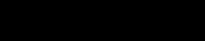
Proof: From Proposition 5 we obtain the identity

are uniformly bounded on as desired. (Note however that the are not CZOs, since modulation does not preserve the CZO class.) Since converges in norm to for Schwartz functions (by dominated convergence), the claim then follows by the usual limiting arguments.
Remark 17 The corresponding question about pointwise almost-everywhere convergence is the Carleson–Hunt theorem, which is quite difficult. Whenan example of Kolmogorov shows that both norm convergence and almost-everywhere convergence can fail. In higher dimensions, the norm convergence for
is true by Plancherel’s theorem, but a surprising result of Fefferman shows that it fails for
. The almost everywhere convergence problem remains open (and is considered very difficult) in higher dimensions.
Exercise 18 Letbe two CZOs with the same kernel
such that
for all
and
. Now observe that
is an absolutely continuous measure, and use the Radon–Nikodym theorem.)
Exercise 19 Show that if we redefine the notion of a CZO by weakening the hypothesis offor some
, then Corollary 14 remains unchanged (but with an operator norm of
instead of
. In particular this apparent expansion of the notion of a CZO does not in fact increase the class of CZOs (up to changes in the implied constants).
— 3. Bounded mean oscillation —
Let us now study what a CZO does on the endpoint space  . At first glance things are rather bad; not only is unbounded on in general, is not even known yet to be defined on a dense subset of . Nevertheless, a closer inspection of things will show that actually does have a fairly reasonable definition on , up to constants.
Let us try to define  for
 directly. A naive implementation of the kernel formula

near , and near infinity, since the decay (4) is not strong enough to give absolute integrability in either case. Localizing to be supported away from helps with the first problem, but not the second. But suppose we instead looked at the difference  between at two values. Then we formally have

 , the expression
 decays like
 as
 , and so the integral will be absolutely integrable as long as vanishes near and
 . At the other extreme, if is compactly supported, then it lies in and there is no difficulty defining
 (up to the usual measure zero ambiguities).
Motivated by this, let us make the following definitions. We say that two functions  are equivalent modulo a constant if there exists a complex number such that
 for almost every ; this is of course an equivalence relation. Given , we define to be the equivalence class associated to the function

 is any ball which contains both and ; it is not hard to see that the right-hand side is well-defined (in particular, the integral is absolutely convergent) and is independent (modulo a constant) of the choice of
 , and that remains linear. One can also check that this definition is consistent (modulo a constant) with the existing definition of on (or on
 ) on the common domain of definition (i.e.
 or
 ).
Because is only defined modulo a constant, we cannot meaningfully control it in standard norms such as . However, there is a norm which is suitable for this type of function.
Definition 20 (Bounded mean oscillation) Letbe a function defined modulo a constant. The
(or Bounded Mean Oscillation) norm of
where
the space of all functions with finite

It is not hard to verify that this is indeed a norm (but note that one has to quotient out by constants before this is the case!), and that is a Banach space. One can also easily check using the triangle inequality that

 ranges over constants; thus the statement
 is equivalent (up to changes in the implied constant) to the assertion that for any ball there exists a constant
 such that
 , thus deviates from by at most
 on the average.
It is not hard to see that contains , and that  . But it also contains unbounded functions:
Exercise 21 Verify that the functionis in
The primary significance of for Calderón–Zygmund theory is that it can serve as a substitute for  , on which CZOs are often ill-behaved. Consider for instance the Hilbert transform applied (formally) to the signum function
 . The resulting function is not bounded, but lies in :
Exercise 22 Verify that using the previous definitions,modulo constants.
This phenomenon applies more generally to all CZOs:
Proposition 23 (CZOs mapand

Proof: We can normalize  . By definition of the norm, it suffices to show that for every ball there exists a constant such that
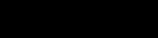
By translation and dilation symmetry we may take  . We split
 . Since is bounded on , we have

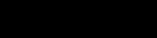
. For the “global” part, observe that for  we have

. But by (6) we have  ; since is bounded by , we thus see that
 , and so

In order to exploit this proposition, we need to understand to what extent BMO bounds on a function control its size. The basic insight here is that BMO bounds are “almost as good as” control for many purposes, despite the logarithmically unbounded members of BMO such as  .
Let us first work informally. Let be a real-valued BMO function, normalized so that  , thus
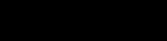
. By Markov’s inequality, this means that 
. Note that this bound is only non-trivial for  , otherwise the trivial bound of
 is superior. It asserts, for instance, that only exceeds its average by (say)
 on at most
 of any given ball.
It turns out that one can iterate the above fact to give far better estimates in the limit  that (8) initially suggests. This is because of a basic principle in harmonic analysis: bad behavior on a small exceptional set (such as of any given ball) can often be iterated away if we know that the exceptional sets are small at every scale. Roughly speaking, this principle allows us to say that only exceeds its average by
 on at most of of a given ball (i.e. on at most
 of the ball), exceeds its average by
 on at most
 , and so forth, leading to a bound of the form (8) which tails off exponentially in rather than polynomially. More precisely, we have
Proposition 24 (John–Nirenberg inequality) Let. Then for any ball
for all
depending only on

Proof: We can normalize  . For each let
 denote the best constant for which we have

is a ball and is a real-valued function with BMO norm . From (8) and the trivial bound of we have the bounds 

We shall do this by a variant of the Calderón–Zygmund decomposition. We’ll need a moderately large quantity  to be chosen later, and assume that
 . Let be any ball, and let
 . Then we have

 . Let be small, and let be any compact set in such that


 are a finite collection of balls intersecting such that
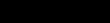 and



intersects , which is contained in , we can conclude that  if we choose
 large enough.
Observe that  is pointwise bounded almost everywhere by
 (by the Lebesgue differentiation theorem), and so

we see that  , and hence



is arbitrary we can remove it. Taking suprema over all and we conclude the recursive inequality 
sufficiently large depending on , and iterating starting from the trivial bound  , we obtain the claim.
Using the distributional characterization of the norms, we conclude
Corollary 25 (Alternate characterization of BMO norm) For anyand all locally integrable

Exercise 26 Prove this corollary.
Exercise 27 Show that Corollary 25 is in fact true for all.
One consequence of this corollary, when combined with the Calderón–Zygmund decomposition, is that the norm serves as a substitute for the norm as far as log-convexity of Hölder norms is concerned:
Lemma 28 Letand
. Then
and

Proof: By rescaling one can normalize  . Let us understand the size of the distribution function
 . From the bound we already have

We can get a better bound for large as follows. Applying the version of the Calderón–Zygmund decomposition at level , we can find a collection of disjoint dyadic cubes with  , such that
 almost everywhere outside of
 , and such that
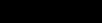 on each cube . If we let be a ball containing of comparable diameter, we then easily verify that
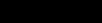 also, and thus
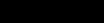 . From the John–Nirenberg inequality we thus see that

large enough; summing over we conclude that 
. Combining this with the bound for small and using the distributional formula for the  norm we obtain the claim.
Because of this, we can also use as a substitute for for real interpolation purposes. For instance, let be a CZO and  . It is now easy to check that is restricted type . Indeed, for any sub-step function of height and width
 , the boundedness on gives



, which is the restricted type. Further interpolation then gives strong type. (Note that these arguments are essentially the dual of those which establish weak-type for  ; in particular, note how the Calderón–Zygmund decomposition continues to make an appearance.)
Exercise 29 (Lacunary exponential sums lie in BMO) Letbe a sequence of non-zero frequencies in
which are lacunary in the sense that
for all
. Let
be a sequence of complex numbers which obeys the
bound
. To avoid issues of convergence let us assume that only finitely many of the
are non-zero. Let
be the exponential sum
If
is an interval in
is a bump function adapted to
for some constant
. (Hints: split the
, and the low frequencies where
. For the high frequencies, forget about
. For the low frequencies, choose
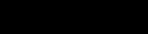


Exercise 30 (Dyadic BMO) Given anyand any locally integrable
, define the dyadic BMO norm
of
where
. Show that we have the John–Nirenberg inequality
for all
, and in particular
for all
as well.)



Exercise 31 (BMO and dyadic BMO) For any locally integrablebut that the converse inequality is not true. On the other hand, if we let
be the shifted dyadic meshes from the previous week’s notes, and set
to be the associated shifted dyadic BMO norms, show that


Exercise 32 (John–Nirenberg via Bellman functions) Letbe the function
. Use a Bellman function approach to establish the John–Nirenberg type inequality
for some absolute constants
, all intervals
with
.

Exercise 33 (Sharp function, I) For any locally integrable function, define the function
as
where the supremum ranges over all balls containing
Show that we have the pointwise bound



Exercise 34 (Sharp function, II) Let, and let
for at least one
for at least one
. Use the Hardy–Littlewood maximal inequality to show that for any sufficiently large
, that
From this and a Vitali covering lemma or Calderón–Zygmund decomposition argument, conclude the good
and then (by taking
for all
. Use this to give an alternate proof of Lemma 28.



— 4. Multiplier theory —
An important subclass of CZOs are given by certain types of Fourier multipliers. (We also have spatial multipliers  , but their behavior is much more elementary to analyze thanks to Hölder’s inequality; for instance, a spatial multiplier
 is bounded on if and only if the symbol
 is in , and indeed the operator norm of the former is the sup norm of the latter.)
Definition 35 Ifis a tempered distribution we define the Fourier multiplier
on Schwartz functions
by the formula
We refer to the function
.

Note that if is Schwartz, then so is  , and that is enough to make
 a tempered distribution, and so
 is well-defined as a tempered distribution. If is bounded, we observe from Plancherel’s identity that

in this case. Indeed it is not hard to show that in fact 
The partial derivative operator  is a Fourier multiplier with symbol
 . More generally, any constant-coefficient differential operator
 , where
 is a polynomial, has symbol
 ; thus one can formally view
 in as representing the vector-valued operator
 . The translation operator
 is a Fourier multiplier with symbol
 , thus we formally have
 . A convolution operator
 , with a distribution, is a Fourier multiplier with symbol
 ; conversely, every Fourier multiplier is a convolution operator with the distribution
 . The Hilbert transform is a Fourier multiplier with symbol
 , thus
 .
Let  . We say that is an multiplier if extends to a bounded linear operator on , and in that case denote
 to be the operator norm of on
 . Thus for instance the
 norm is the same as the norm. At first glance, it seems one can say quite a lot about these quantities; for instance, since the adjoint of is easily seen to be
 , which has the same operator norm as , we see that


multipliers are bounded (though the converse turns out to be false, as we shall see later). The space of multipliers turns out to be a Banach algebra, thus the norm is a Banach space norm and furthermore 
norm is invariant under translations, modulations, and dilations: 
 we can check that

 is an affine transformation rather than a linear one.
Thus for instance, by modulating the Hilbert transform we see that

, which by Riemann–Stieltjes integration and Minkowski’s inequality shows that 
has bounded variation, where 
Exercise 36 Show that if
Exercise 37 Letand
be
is also an
(Hint: it may help to first establish the cases when
or
.)

For  or
 , it is also not hard to show that

is absolutely integrable; with a little more work one can also show that is unbounded on and when  does not lie in
 , although this is a little tricky. Thus for we have (by Riesz–Thorin again)

One consequence of this is that if is a bump function adapted to  for some fixed bounded domain and some arbitrary affine linear transformation , then is an multiplier with
 for all .
Suppose a multiplier on does not depend on the final coordinate  , thus

 . Then the -dimensional Fourier multiplier and the
 -dimensional Fourier multiplier
 are related by the identity

 and Schwartz , where
 is the slice

 is in
 , then is in
 with

Of course, most multipliers on do depend on the final coordinate . Nevertheless we can obtain a partial generalization of (11) for these more general multipliers:
Theorem 38 (De Leeuw’s theorem) Ifis continuous, then
for any
Proof: By translation invariance we can take  . For any , let
 be the linear transformation


. We observe from the hypothesis that is continuous that  pointwise, where
 is the (non-invertible) projection



 are Schwartz functions, we see from Hölder’s inequality that

and using Plancherel and dominated convergence on the left-hand side (using the pointwise convergence, as well as the boundedness of ) we conclude 
One consequence of de Leeuw’s theorem is that we expect multiplier theory on higher dimensions to be harder than multiplier theory for lower dimensions.
One can view de Leeuw’s theorem as a transference theorem, transferring a bound on one space () to another ( ), basically by exploiting the fact that there was a projection from to . For a result of similar flavor, see Exercise 39.
Exercise 39 (Transference theorem for) If
is bounded, define the multiplier
by the formula
where we use the Fourier transform on the torus
,
We then define
to be the
operator norm of
Let
. (Hint: take functions
, extend them periodically to
), apply
.)


Despite these encouraging initial results, it appears very difficult to decide in general whether any given multiplier lies in or not for any other than . For instance, the question of determining the precise values of and  for which the multiplier
 is an multiplier is not fully resolved in three and higher dimensions; this problem is known as the Bochner–Riesz conjecture, which we will not discuss in detail here. Broadly speaking, the difficulty with the Bochner–Riesz conjecture is that the symbol
 is singular on a large, curved set (in this case, the sphere), which necessarily leads to some delicate and still incompletely understood geometric issues (most notably the Kakeya conjecture, which we will also not discuss here).
However, one can do a lot better if the multiplier has no singularities, or is only singular at one point (such as the origin). For instance, if is Schwartz, then is definitely in , and so lies in for all . Note from (9) that any dilate, translate, and/or modulation of a Schwartz function is then also in uniformly in the dilation, translation, and modulation parameters.
Now we address multipliers which only have singularities at the origin.
Theorem 40 (Hörmander–Mikhlin multiplier theorem) Letfor all
and
. (In particular
.) Then
for all

Remark 41 It is possible to use less regularity thanderivatives here, but in practice this type of control is sufficient for many applications. The conditions (12) are essentially asserting that
, although it essentially allows different annuli to behave independently. For instance, if
is a bump function adapted to the annulus
are arbitrary signs, then
obeys the homogeneous symbol estimates of order
.
Proof: The multiplier is already bounded on . Formally, we know that is a convolution operator:  , but we run into the formal difficulty that need not be locally integrable. To compute things rigorously it is convenient to use the Littlewood–Paley decomposition. Let
 be a fixed bump function which equals one on the ball
 and is supported on the ball
 , and write

 . Then we have the partition of unity

 , and hence we have the pointwise convergent sum

 . Using Plancherel and dominated convergence we conclude that
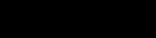
, where the sum is conditionally convergent in the sense. In particular for any  we have

 are also bounded and compactly supported with disjoint supports. We can write


 are bounded with compact support; we omit the details. Now observe that
 is supported on the annulus
 , and multiple applications of the Leibnitz rule give us the bounds

. From the  case of this bound and the triangle inequality we obtain the bound

 times (using the identity
 ) we obtain the bound

 , and hence


 factor essentially just contributes an extra factor of
 to the analysis, and we end up with

, the series  is convergent in
 to a kernel
 obeying the bounds


are bounded with disjoint support. By a monotone convergence argument (noting that is bounded on ) the same is true when are with compact support.
The bounds (13) (and the fundamental theorem of calculus) ensure that  is a singular kernel, and (14) shows that is a CZO with kernel . Thus, by Corollary 14, is of strong-type with an operator norm of
 for all , and the claim follows.
Note that the Hörmander–Mikhlin multiplier theorem includes the boundedness of the Hilbert transform for as a special case, since the multiplier  certainly obeys the symbol estimates. Another useful instance of the theorem is to conclude that the homogeneous fractional derivative operators
 , with symbol
 and
 real, are also bounded on , with an operator norm of
 (in particular, it grows at most polynomially in ). This fact turns out to be very useful when one wishes to use Stein interpolation involving fractional differentiation operators
 . A similar argument also applies to the inhomogeneous fractional derivative operators
 with symbol
 . (The factor of
 is of course irrelevant here and the same results hold if this factor is dropped. Indeed, in PDE it is customary to drop the from the definition of the Fourier transform so as not to see these factors then arise from differential operators.)
Another example of multipliers covered by this theorem are the Riesz transforms  for
 , with symbol
 . These symbols are easily verified to obey the homogeneous symbol estimates and are thus in with norm for all . The significance of the Riesz transforms is that they connect general second order derivatives to the Laplacian; indeed from Fourier analysis we quickly see that
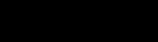
 and Schwartz . In particular, since
 is bounded on , we obtain the elliptic regularity estimate

and all . In a similar vein, we can show that 
 , Schwartz , and , where
 is the Fourier multiplier with symbol
 .
More generally, any multiplier which is homogeneous of degree zero (thus  for all ), and smooth on the sphere
 , obeys the homogeneous symbol estimates and is thus in for all .
The Fourier multipliers covered by the Hörmander–Mikhlin multiplier theorem are essentially special cases of the pseudodifferential operators of order , which we shall discuss in later notes.
— 5. Vector-valued analogues —
In the above discussion we considered only scalar-valued (complex-valued) functions, and scalar-valued operators with scalar kernels . However, it is possible to generalize basically all of the above discussion to vector-valued cases, in which the functions take values in a Hilbert space, and the kernel takes values in the bounded linear operators from one Hilbert space to another. We rapidly present these generalizations here; as it turns out only some notational changes need to be made. We will then give an important application of this generalization, namely the Littlewood–Paley inequality.
Let be a Hilbert space. For  , we let
 be the space of measurable functions
 such that
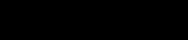
 in the usual manner. One can (rather laboriously) rederive most of the scalar theory to this vector-valued case (mostly by replacing absolute values with norms, and any scalar form
 with the inner product
 ). For instance, one can verify the duality relationship

and  . Also, the real interpolation theory continues to be valid in this setting (the basic reason being that the layer-cake decompositions, which depend only on the magnitude of the underlying function, continue to be valid).
Observe that if is absolutely integrable on some set , thus  , then one can define the vector-valued integral
 in several ways, for instance by using duality

, we can compute averages  for balls or cubes .
Let  denote the bounded linear operators of to
 , with the usual operator norm.
Definition 42 (Vector-valued singular kernels) Letbe Hilbert spaces. A singular kernel from
(defined away from the diagonal
for
and
for some Hölder exponent



Definition 43 (Vector-valued Calderón–Zygmund operators) A Calderón–Zygmund operator (CZO) fromwhich is bounded,
and such that there exists a singular kernel
whenever
is compactly supported, and

One can then repeat the derivation of Corollary 14 more or less verbatim to show that vector-valued Calderón–Zygmund operators continue to be bounded from  to
 with bound . Note that the constants never depend on the dimension of and , and indeed this dimension may be infinite.
An important application of vector-valued Calderón–Zygmund theory is the Littlewood–Paley inequality.
Proposition 44 (Upper Littlewood–Paley inequality) For each integer, let
be a bump function adapted to an annulus
. Then for any
and for any
for
where the sum in the left is conditionally convergent in


Proof: By monotone convergence it suffices to prove the claim assuming that only finitely many of the are non-zero. (This step is not strictly necessary, but it lets us avoid unnecessary technicalities in what follows.) It suffices to prove the first claim, as the second follows from a standard duality argument.
We consider the vector-valued operator  defined by


 , we quickly see from Plancherel’s theorem that is strong-type
 with operator norm . Next, we observe that has a vector-valued kernel

 to
 in the obvious manner. But as in the proof of the Hörmander–Mikhlin multiplier theorem we have


Corollary 45 (Two-sided Littlewood–Paley inequality) For each integer. Then for any

Proof: By density (and the preceding proposition) it suffices to prove this when is Schwartz.
From the preceding proposition we already have the upper bound; the task is to establish the lower bound. Let  be bump functions adapted to a slightly wider annulus than , which equal on the support of . Writing
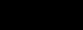
 is also adapted to the same annulus as , and that we have the partition of unity
 . This leads to the identity
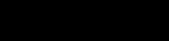
is Schwartz, and hence by (18) we obtain 
The quantity  is known as a Littlewood–Paley square function of . One can view
 as the component of whose frequencies have magnitude
 . The point of the inequality is that even though each component may individually oscillate, no cancellation occurs between the components in the square function. This makes the square function more amenable than the original function when it comes to analyze operators (such as differential or pseudodifferential operators) which treat each frequency component in a different way.
Exercise 46 (Continuous Littlewood–Paley inequality) For every, let
be a function obeying the estimates
for all
, all
, and some
for
, improve this bound to



— 5.1. An alternate approach via Khintchine’s inequality —
One can avoid dealing with vector-valued CZOs by instead using randomized signs as a substitute. The key tool is the following inequality, which roughly speaking asserts that a random walk with steps  is extremely likely to have magnitude about
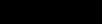 , and can be viewed as a variant of the law of large numbers:
Lemma 47 (Khintchine’s inequality for scalars) Letbe independent random signs, drawn from
with the uniform distribution. Then for any
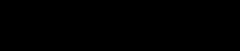
Proof: By the triangle inequality it suffices to prove this when the  are real. When we observe that

 has expectation when
 and when
 . This proves the claim for . By Hölder’s inequality this gives the upper bound for
 and the lower bound for
 . Hölder also shows us that the lower bound for will follow from the upper bound for , so it remains to prove the upper bound for .
We will use the “exponential moment method”. We normalize 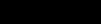 . Now consider the expression
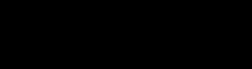

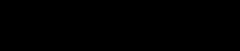
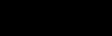
 )
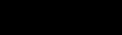
norm.
Remark 48 It is instructive to prove Khintchine’s inequality directly for even exponents such as.
Corollary 49 (Khintchine’s inequality for functions) Letfor some

Proof: Apply the above inequality to the sequence  for each
 and then take norms of both sides.
This gives the following alternate proof of Proposition 44. Once again we may restrict to only finitely many of the being non-zero. Observe that for arbitrary choices of signs  , that the sum
 obeys the homogeneous symbol estimates of order . Thus by the Hörmander–Mikhlin theorem we have

. Taking expectations and using Khintchine’s inequality we obtain the claim.
Exercise 50 (Chernoff’s inequality) Iffor all
. (Hint: look at
for a real parameter

Exercise 51 (Marcinkiewicz–Zygmund vector extension) Letwe have
(Hint: reduce to finite summation and use Khintchine’s inequality.)

Exercise 52 (BMO Littlewood–Paley inequality) For each integer; assume that all but finitely many of the
are non-zero. Let
(It is possible to remove the hypothesis that finitely many of the
; in particular it will only be defined modulo a constant.)

Exercise 53 (Zygmund’s inequality) For each positive integerbe an integer with
, and let
finite. Show that
and in particular that
for all
, show that
and in particular that
for all
.






Discussion
Sign in to join the discussion.